STCE Newsletter

1. An early solar cycle minimum?
2. PROBA2 Observations (29 Jan 2018 - 4 Feb 2018)
3. Basic Solar Physics Seminars
4. Review of solar and geomagnetic activity
5. The International Sunspot Number
6. Geomagnetic Observations at Dourbes (29 Jan 2018 - 4 Feb 2018)
7. Review of ionospheric activity (29 Jan 2018 - 4 Feb 2018)

An early solar cycle minimum?

For the last couple of years, signs have been piling up that our star is entering the minimum phase of its activity cycle. There's the obvious decrease in the monthly international sunspot number as compiled by SILSO (http://sidc.be/silso/ ), but there are other, less-known features which confirm this evolution and even hint that the next solar cycle minimum may be even a bit earlier than expected. These have been mentioned in past STCE news items: the first spots of cycle 25 (http://www.stce.be/node/359 , http://www.stce.be/news/414/welcome.html ) observed in December 2016 and January 2018, the increasing number of spotless days (http://www.stce.be/news/406/welcome.html , http://sidc.oma.be/silso/spotless ), and the high number of polar faculae observed since the second half of 2015 (http://www.stce.be/news/318/welcome.html , http://www.stce.be/news/333/welcome.html ).

In this news item, analysis of the solar radio emission suggests that the next solar cycle minimum might be closer upon us than what we would expect from the sole analysis of sunspot data.

Besides the sunspot number, another well-known indicator of solar activity is the F10.7 index, which is the flux density of the Sun observed in the radio domain at a frequency of 2800 MHz (corresponding to a wavelength of 10,7 cm). The Penticton Observatory, on the west coast of Canada, currently provides the measurements of this index (http://www.spaceweather.gc.ca/solarflux/sx-5-en.php ). It corresponds, in principle, to the emission of the quiet Sun (outside flaring events), but it may sometimes be "polluted" by long duration radio counterparts of flares. A long time series is available since 1947, when the first systematic observations began and this is, besides the Sunspot index, one of the longest records of solar activity. When adjusted for the varying distance to the Sun, this index provides interesting clues on the behaviour of the Sun as time goes by. This is the data set we will refer to from now on.

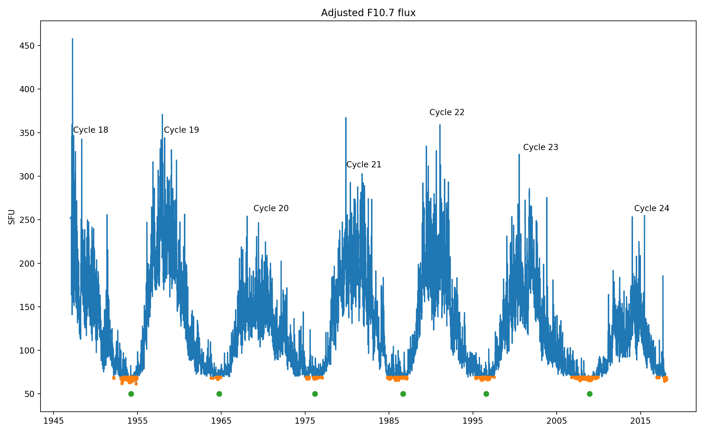
The figure above shows the daily adjusted measurements of the solar flux density in Solar Flux Units (1 SFU = 10^(-22) W.m^(-2).Hz^(-1) ), from 1947 till the end of January 2018. The green dots mark the time of the official minima of the different sunspot cycles (source https://en.wikipedia.org/wiki/List_of_solar_cycles ). The orange dots highlight the time period when the flux drops below or is equal to 70 SFU. This threshold might seem somewhat arbitrary, but it corresponds to the peak in the histogram of the measurements, meaning it is the most frequent value in the series despite being so low.

From this figure, it can be seen that months with values below 70 SFU are clustered around the official solar minimum of the different cycles. If one counts how many days per month are below that threshold since the beginning of the observations, we obtain a distribution of values/month, shown in the figure underneath. There, we can see a collection of box plots, which describe graphically the "shape" of the distributions. Hence, it was chosen to divide the ensemble in chunks of five days ("binning"). The first one to the left for example, describes how the months for which there were 1 to 5 days with the F10.7 index below or equal to 70 SFU, are distributed in time around solar minimum (in days). The orange mark is the median, the limit of the box represents the 1st and 3rd quartiles, and the whiskers (the "T") are used as a threshold for determining outliers (indicated by circles). More details on quartiles can be found in Wikipedia (see https://en.wikipedia.org/wiki/Interquartile_range ). In our example (1-5 days/month), most of these months occur a bit less than 300 days before minimum, with a rather large margin from about 500 days before to 150 days after the cycle minimum. Months with values below 70 SFU happening 800 days before or 400 days after cycle minimum are rare ("outliers").

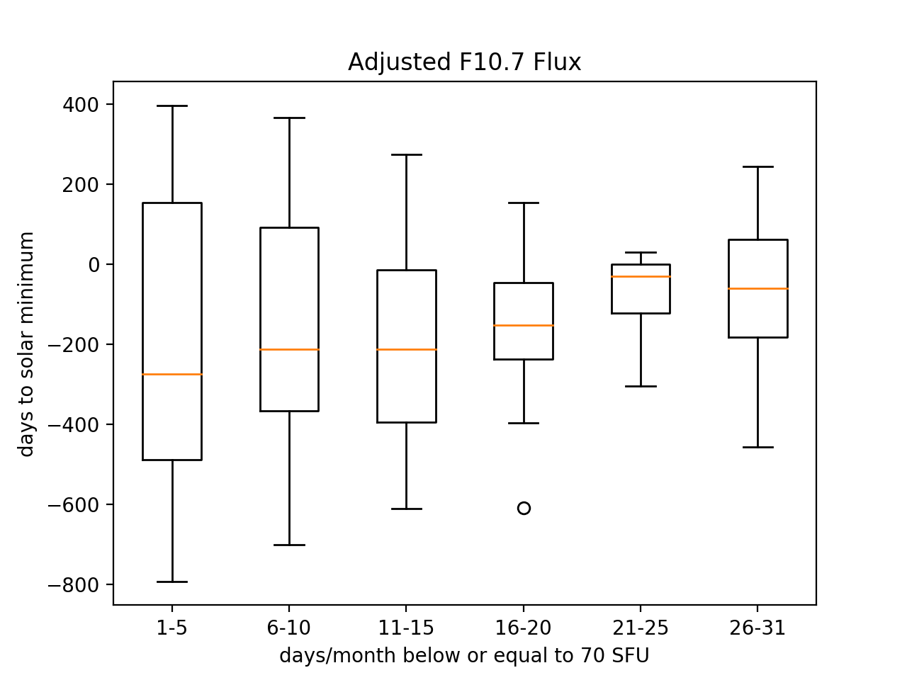
From the above figure, we can also see that values below or equal to 70 SFU are predominantly observed prior to the cycle minimum (each box plot is skewed towards negative values). Moreover, months having many days with values below 70 SFU are more frequent close to the minimum of the cycle.
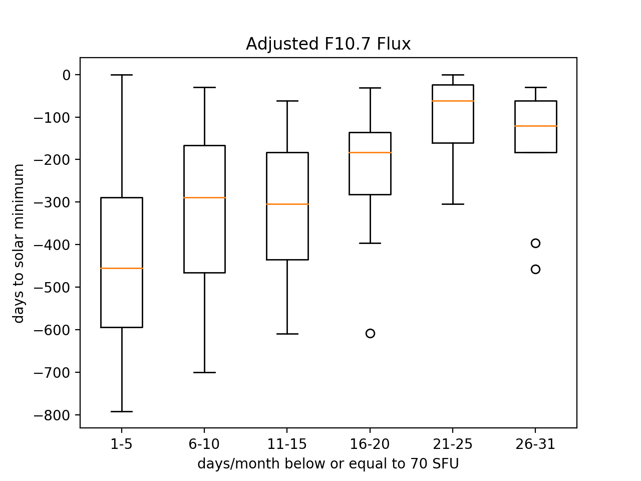
If we redraw these box plots by limiting ourselves to periods prior to the minimum, we then obtain the plot shown underneath. There, we see a more pronounced trend: as the number of days per month below 70 SFU increases, we are closer to the minimum of the solar cycle.

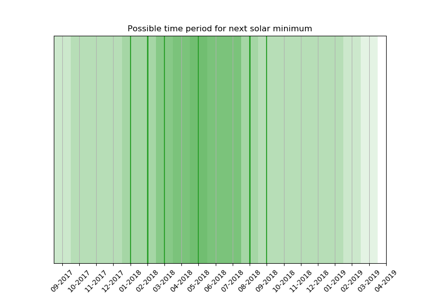
Of course, even during a cycle minimum, solar activity can vary significantly from one month to the other. Moreover, the uncertainty margins in the plots are rather large. Can we then reliably derive from these observations a hint for the timing of the next minimum? If one assumes that the current cycle will behave like the ones observed in the past (Note 1), we can project the results shown in the above figure to the current situation.
During this solar cycle transit (cycle 24-25), the observed F10.7 values dropped below 70 SFU for the first time in December 2016 (4 days), with the number alternating between 0 and a full month, the latter being the case for January 2018. We can then, from the limits of the boxes and median values of the foregoing figure, estimate the corresponding time intervals for the upcoming minimum. This is shown in the figure underneath. Intervals are green shaded areas which overlap. The "darkest" green area shows the most likely period where the minimum could occur: in this case between March and July 2018. The vertical green lines are the median values of each deduced time interval, with one falling in the middle of the aforementioned period, i.e. in May 2018. Note the uncertainty in the prediction with March 2019 as an upper limit. With these timings, SC24 would turn out to be a rather short cycle lasting barely 10 years.

In summary, the main purpose of this exercise was to illustrate the evolution of the solar radio flux density during the period of the sunspot minimum. Assuming that the current solar activity behaviour is similar to that in the past, the next minimum might be right around the corner. However, as past experience has shown so often, our star manages to surprise us time and time again. So let’s wait a little and see how it turns out this time.

This news item was prepared by Christophe Marqué (STCE / Humain Solar Radio Observatory) with the help and comments from Jan Janssens (STCE).

Note 1 - The previous minimum (between solar cycles 23 and 24) was notoriously atypical for its duration, and would probably not have been forecast correctly based on data prior to cycle 23. Here, the values from the cycle 23-24 minimum have been included.

PROBA2 Observations (29 Jan 2018 - 4 Feb 2018)

Solar Activity

Solar flare activity fluctuated between very low and low during the week.
In order to view the activity of this week in more detail, we suggest to go to the following website from which all the daily (normal and difference) movies can be accessed: http://proba2.oma.be/ssa
This page also lists the recorded flaring events.

A weekly overview movie can be found here (SWAP week 410).
http://proba2.oma.be/swap/data/mpg/movies/weekly_movies/weekly_movie_2018_01_29.mp4

Details about some of this week’s events, can be found further below.

If any of the linked movies are unavailable they can be found in the P2SC movie repository here
http://proba2.oma.be/swap/data/mpg/movies/

Sunday Feb 04

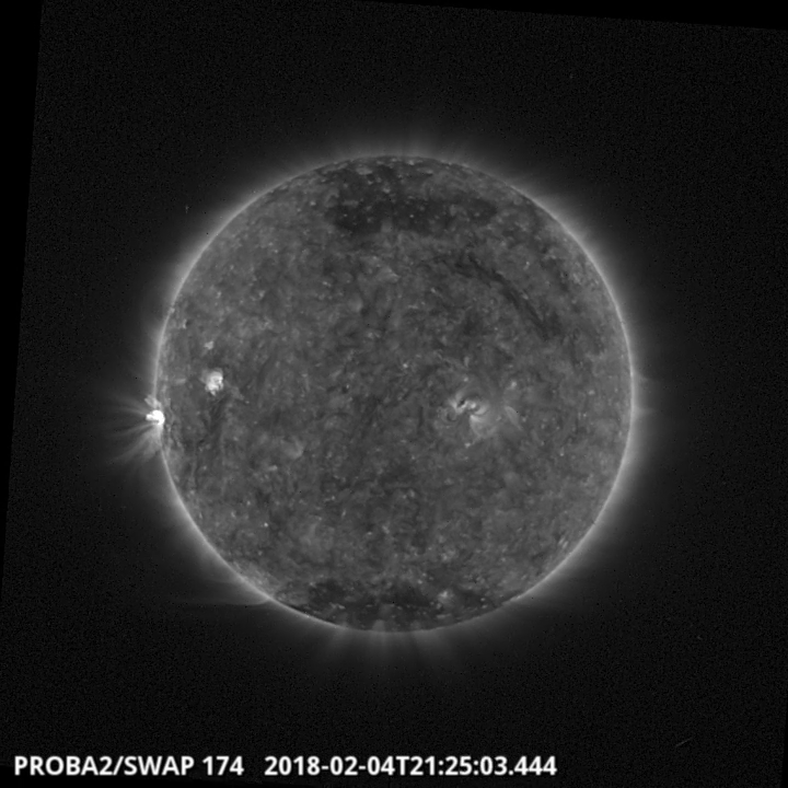
A C-class (C1.1) flare, associated with NOAA AR 2699 (located in S09E80), was observed by SWAP on 2018-Feb-04. The flare is visible on the east limb of the solar disk in the SWAP image above at 21:25 UT. This flare has been followed by a series of B-class flares.

Basic Solar Physics Seminars

During the sixth of a series of seminars on the basics of solar and heliospheric physic, an overview of observational methods and instruments was given. David Berghmans spoke about EUV and X-ray imagers, coronagraphs, heliospheric imagers and radiometers.
Watch the seminar: https://events.oma.be/indico/event/39/

The seventh seminar by Andrei Zhukov reviewed solar eruptive phenomena (flares and coronal mass ejections) were reviewed and their physics. These solar storms are important because they can disturb the Earth environment.
Watch the seminar: https://events.oma.be/indico/event/40/

Review of solar and geomagnetic activity

SOLAR ACTIVITY

Solar activity was very low.
No sunspot groups were observed at the beginning of the week, until NOAA active region (AR) 2967 appeared on 31 January with beta magnetic field configuration, became alpha on 1 February and decayed into an H-alpha plage on 2 February.
NOAA AR 2698 rotated over the east limb on 3 February (alpha magnetic field configuration) and decayed into a plage the day after. These two ARs did not produce any flare above B-class.
On 4 February NOAA AR 2699 rotated into view (alpha magnetic field configuration), it produced a C1.1 flare peaking at 20:24 UT (4 February).

Several small diffuse coronal holes (negative polarity) and the extension of the positive northern polar coronal hole (CH) transited the central meridian.
No earth-directed CMEs were observed throughout the week.
The greater than 10 MeV proton flux was at nominal levels.

GEOMAGNETIC ACTIVITY

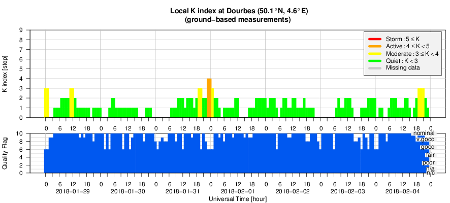
The earth environment was under the influence of a weak high speed solar wind stream on 31 January - 1 February (reaching 460 km / s and 9 nT, producing K = 4) and 4 - 5 February (reaching 450 km/s and 9 nT, producing only K = 3).

The International Sunspot Number

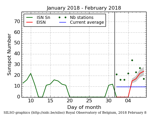
The daily Estimated International Sunspot Number (EISN, red curve with shaded error) derived by a simplified method from real-time data from the worldwide SILSO network. It extends the official Sunspot Number from the full processing of the preceding month (green line). The plot shows the last 30 days (about one solar rotation). The horizontal blue line shows the current monthly average, while the green dots give the number of stations included in the calculation of the EISN for each day.

Geomagnetic Observations at Dourbes (29 Jan 2018 - 4 Feb 2018)

Review of ionospheric activity (29 Jan 2018 - 4 Feb 2018)

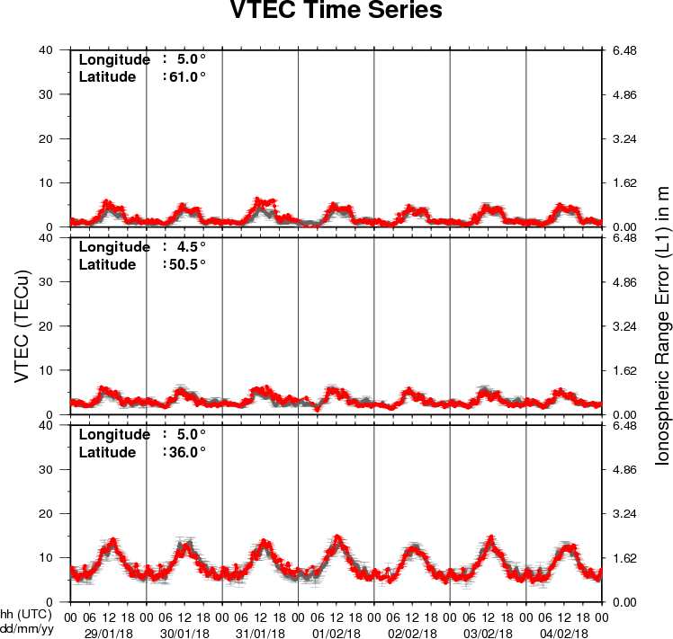
The figure shows the time evolution of the Vertical Total Electron Content (VTEC) (in red) during the last week at three locations:
a) in the northern part of Europe(N61°, 5°E)
b) above Brussels(N50.5°, 4.5°E)
c) in the southern part of Europe(N36°, 5°E)
This figure also shows (in grey) the normal ionospheric behaviour expected based on the median VTEC from the 15 previous days.

The VTEC is expressed in TECu (with TECu=10^16 electrons per square meter) and is directly related to the signal propagation delay due to the ionosphere (in figure: delay on GPS L1 frequency).
The Sun's radiation ionizes the Earth's upper atmosphere, the ionosphere, located from about 60km to 1000km above the Earth's surface.The ionization process in the ionosphere produces ions and free electrons. These electrons perturb the propagation of the GNSS (Global Navigation Satellite System) signals by inducing a so-called ionospheric delay.

See http://stce.be/newsletter/GNSS_final.pdf for some more explanations ; for detailed information, see http://gnss.be/ionosphere_tutorial.php