STCE Newsletter

1. Quo vadis, magnetic pole?
2. Attention Attention - New Space Weather Courses are launched
3. Review of solar and geomagnetic activity
4. PROBA2 Observations (12 Jun 2023 - 18 Jun 2023)
5. International Sunspot Number by SILSO
6. Noticeable Solar Events
7. Geomagnetic Observations in Belgium
8. The SIDC Space Weather Briefing
9. Review of Ionospheric Activity

Quo vadis, magnetic pole?

The magnetic field of the Earth is believed to be generated by convection in the outer core through a dynamo effect ("geodynamo"): fluid motion within a pre-existing magnetic field creates electric currents, which in turn induce a magnetic field that reinforces the pre-existing magnetic field. The resulting magnetic field resembles a dipole field, with the magnetic axis inclined by about 11 degrees to the Earth's rotational axis, and with also an off-set from the Earth's centre by 540 km to the northwest Pacific (SPENVIS - https://www.spenvis.oma.be/help/background/magfield/cd.html#CD ). The solar wind then deforms this field into a drop-shaped configuration, compressed at the sun-facing side, and stretched into a million kilometers long tail at the nightside. Taking into account there are also some non-dipolar contributions from e.g. the ionosphere, the ring current,... the final shape of the true magnetic field is very complex and dynamic. Due to the chaotic movement of the core fluid, the Earth's magnetic field gradually changes over the years. The image underneath shows the horizontal direction of the magnetic field lines at the surface of the Earth for the period 1590-2010. The magnetic North and South poles are shown as blue and red stars, respectively. Note the change in location of the magnetic poles, the clips also show the change in the speed of movement. Where the lines are blue, the magnetic field dips into the Earth, where they are red it emerges from the Earth. The transition from red to blue, where the field lines are horizontal, is called the magnetic equator. Clips are available at CIRES/Geomagnetism - https://geomag.us/info/declination.html

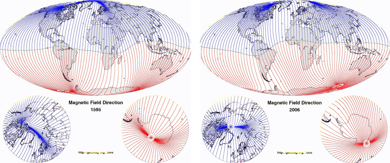
Credits: CIRES/Geomagnetism - https://geomag.us/info/declination.html

To study the geomagnetic field, several models such as for example the International Geomagnetic Reference Field (IGRF ; WDC for Geomagnetism at Kyoto: https://wdc.kugi.kyoto-u.ac.jp/poles/polesexp.html ), have been developed. The coefficients for the equations used in these models are determined experimentally by combining Earth-based and satellite measurements of the geomagnetic field. At the Earth's surface the main field can be approximated by a dipole placed at the Earth's centre and tilted to the axis of rotation by about 11 degrees. This is the so-called centred dipole model. If one takes also the 540 km off-set into account, the model is called the eccentric dipole model. The latter is often used when proxying the true Earth's magnetic field, and the associated poles are called the geomagnetic poles. Nonetheless, one should keep in mind that significant deviations from this dipole field model exist, both in location as in intensity (see BGS - http://www.geomag.bgs.ac.uk/education/earthmag.html ).

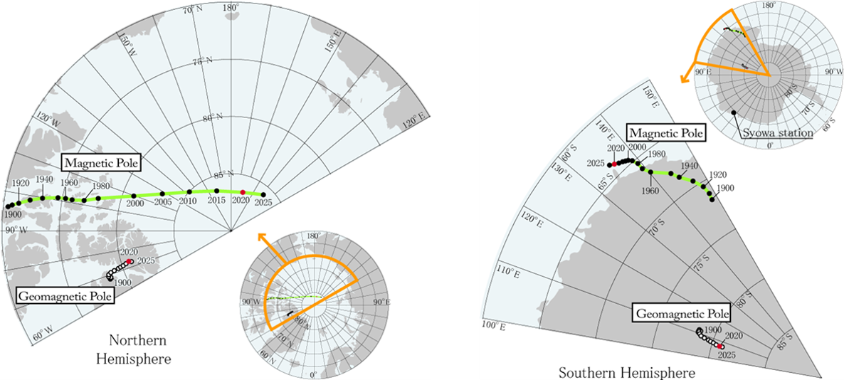
Credits: WDC for Geomagnetism Kyoto - https://wdc.kugi.kyoto-u.ac.jp/poles/polesexp.html

Thus, the location of these (modelled) geomagnetic poles differs from the true magnetic poles, the latter which are located where the magnetic field lines are perpendicularly entering (North pole) or leaving (South pole) the Earth's surface. Also known as the dip poles, these true magnetic poles are not antipodal, unlike their cousins of the dipole centred model. This can be seen in the maps above (WDC Kyoto - https://wdc.kugi.kyoto-u.ac.jp/poles/polesexp.html ) showing the locations for the northern and southern poles. The 2020 location of the North Magnetic Pole is 86.5 North and 162.9 East and the South Magnetic Pole is 64.1 South and 135.9 East (IGRF ; NCEI - https://www.ncei.noaa.gov/news/tracking-changes-earth-magnetic-poles ). From the above maps, it is clear that the location of these poles is not stable. Historic (100+ years) and paleomagnetic records (1 million years) clearly show that, in addition to polarity reversals, the magnetic poles have moved over time scales of decades to millions of years. This is called the "polar wander" (also known as "secular drift"), with the movement of the South Pole not being synchronous with that of the North Pole (Nagarajan 2020: http://dx.doi.org/10.1007/s12045-020-0951-9 ).

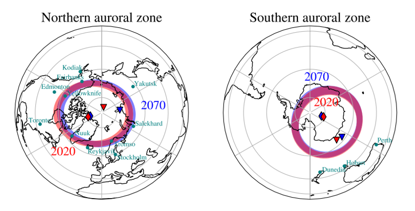
Credits: Maffei et al. 2023: https://www.nature.com/articles/s41598-022-25704-2

Recent decades have seen a remarkable acceleration of this secular drift of the dip pole in the Northern Hemisphere from Arctic Canada toward the coast of Eastern Siberia (Tsyganenko, 2019 - https://doi.org/10.1029/2019GL082159). As of present, the North dip pole has crossed the border between the western and eastern hemispheres, having passed only about 400 km from the North geographic pole. This drift is much smaller for the South dip pole. The effects of this drift of the North magnetic pole severely compromise the precision of direction finding of airport runways in the Northern Hemisphere (the "numbers" at the beginning and end of the runways), as well as navigation at high latitudes, precision surveys and drilling (Nagarajan, 2020). In view of such dramatic displacement, a natural question arises: how large and fast is the associated secular shift of the auroral ovals? Tsyganenko (2019) found that the secular shift of the auroral oval between 1965 and 2020 is about the same as that of the geomagnetic dipole axis, which is much slower than the fastly racing dip pole. In the Southern Hemisphere, the oval shifts are much smaller than in the Northern Hemisphere. Maffei et al. (2023 - https://www.nature.com/articles/s41598-022-25704-2 ) extended the current evolution to 2070, when the North dip pole would be located near Siberia. In the map above, auroral zones ("quiet" space weather conditions) for the 2020 (in red) and 2070 (in blue) epochs are displayed. The red and blue diamonds indicate the location of the geomagnetic poles at 2020 and 2070, respectively. The red and blue triangles indicate the location of the magnetic dip at 2020 and 2070, respectively. They concluded that, under these circumstances, it will be increasingly unlikely to spot aurorae in North American locations with the same latitudes as Edmonton (Canada) and Kodiak (Alaska), while it will be increasingly likely for locations such as Yakutsk, in Russia. Little change is expected for Europe, Australia and New Zealand.

For extreme space weather events, when the auroral ovals expand and move equatorially from their typical 65-70 degrees magnetic latitude to 50-60 degrees magnetic latitude, the results found by Maffei and his collaborators echo those found for the auroral zones. This can be seen in the map below, showing a near-side projection of the regions exposed to severe space weather events ("danger zones") for the 2020 (the orange bands) and 2070 (the cyan bands) epochs. In particular, there is little change in Northern Europe, with the Northern UK, Denmark and Scandinavia still remaining in these high-risk regions in 2070. Most notably, the high-risk band in North America moves northward, resulting in its southern edge shifting from approximately New York City in 2020 to Toronto in 2070. This northward change of the auroral and danger zones over North America will likely cause urban centres such as Edmonton and Labrador City (Canada) to be exposed by 2070 to the potential impact of severe solar activity. In the southern hemisphere, the largest predicted change of the high-risks bands is a motion towards South America in the Southern Atlantic Ocean. In the Indian and Pacific Ocean the changes are modest, with a small drift southward. In particular, the island of Tasmania and Southern New Zealand (including the city of Dunedin), will remain in the same risk region between 2020 and 2070, according to their forecast. To keep in mind: the measured magnetic fields are very sensitive to even small changes in the geodynamo (Livermore et al. 2020 - https://www.nature.com/articles/s41561-020-0570-9 ), which we can't predict, and so it is perfectly possible that within one or two decades the North dip pole is changing its course back to Canada, and all of the above was just a very nice thought experiment.

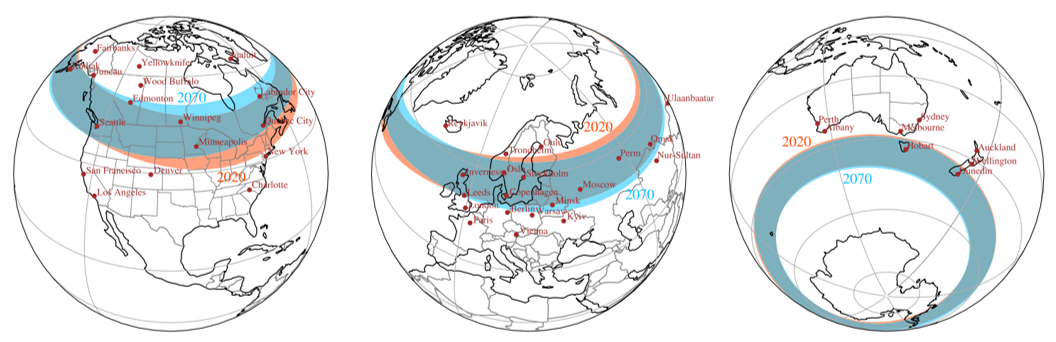
Credits: Maffei et al. 2023: https://www.nature.com/articles/s41598-022-25704-2

Attention Attention - New Space Weather Courses are launched

We are happy to announce the dates of the new STCE Space Weather Courses:

September 18 -20, 2023: Space Weather Introductory Course and post-SWIC on September 26: https://events.spacepole.be/event/170/
December 04-06, 2023: Space Weather impacts on ionospheric wave propagation - focus on GNSS and HF: https://events.spacepole.be/event/173/
January 22-24, 2023: Space Weather Introductory Course and post-SWIC on September 26: https://events.spacepole.be/event/171/

The number of participants for each course is limited to 8.
Fee reductions/waivers are available for priority user groups.

We will (do our best to) serve an excellent course juiced with interesting exercises and learning games.

Welcome!
Elke, Jan, Petra and the STCE experts
P.S. An overview of the courses and activities of the STCE Space Weather Education Center can be found on https://www.stce.be/SWEC

Review of solar and geomagnetic activity

Solar Active Regions (ARs) and flares

Solar flaring activity ranged between low and moderate levels. There was a total of 14 active regions observed on the visible side of the solar disk. At the start of the week, solar flaring activity was at low levels; NOAA AR 3327, NOAA AR 3333 and NOAA AR 3335 were the sources of the majority of the flaring activity. From June 15, the solar flaring activity increased to moderate levels. The largest flare was an M2.5 flare, peaking at 13:53 UTC June 18. This flare was associated with NOAA AR 3336 and also produced a Type II radio burst. This region and others also produced 4 other low level M-class flares between June 15 and June 18.

Coronal mass ejections

There were multiple Coronal Mass Ejections (CMEs) observed over the week, many of which were associated with filament eruptions. One CME was considered to have a possible Earth directed component: A large filament eruption, which stretched from the central meridian to the north-west quadrant observed in SDO/AIA from 17:57 UTC June 17. The bulk of the CME was directed to the northwest and the speed was very slow (350 km/s) but a glancing blow at Earth was predicted possible from June 22.

Coronal Holes

An equatorial negative polarity coronal hole began to cross the central meridian on June 12. Later in the week, two small coronal holes also crossed the central meridian on June 17, one negative and one positive. Both were at high latitudes, in the southern and northern hemispheres, respectively.

Solar Proton flux levels

The greater than 10 MeV GOES proton flux was at nominal levels.

Solar wind near Earth

The solar wind conditions (ACE) at the start of the week, reflected background slow solar wind regime. The solar wind speed varied between 300 and 450 km/s. From around 12:00 UTC on June 15, a Corotating Interaction Region (CIR) was observed, with an increase in the interplanetary magnetic field to values around 20 nT. The solar wind speed increased sharply from 21:00 UT on June 15, with the arrival of the High Speed Stream (HSS), to values above 700 km/s and remained elevated on June 16 and June 17. By the end of the week, the solar wind speed was slowly decreasing and levelled out around 400km/s.

Electron fluxes at GEO

The greater than 2 MeV electron flux was at nominal levels for the first half of the week. It began to increase from June 16 and exceeded the 1000 pfu threshold from June 17. The 24h electron fluence was at normal levels at the start of the week increasing to moderate levels by June 18.

Geomagnetism

At the start of the week the geomagnetic conditions were quiet to unsettled. On June 15 and 16, the level increased to moderate storm conditions globally (NOAA Kp =6) and minor storm conditions locally (K Bel = 5) in response to the CIR and HSS arrivals.
Conditions then returned to quiet to unsettled levels from June 17.

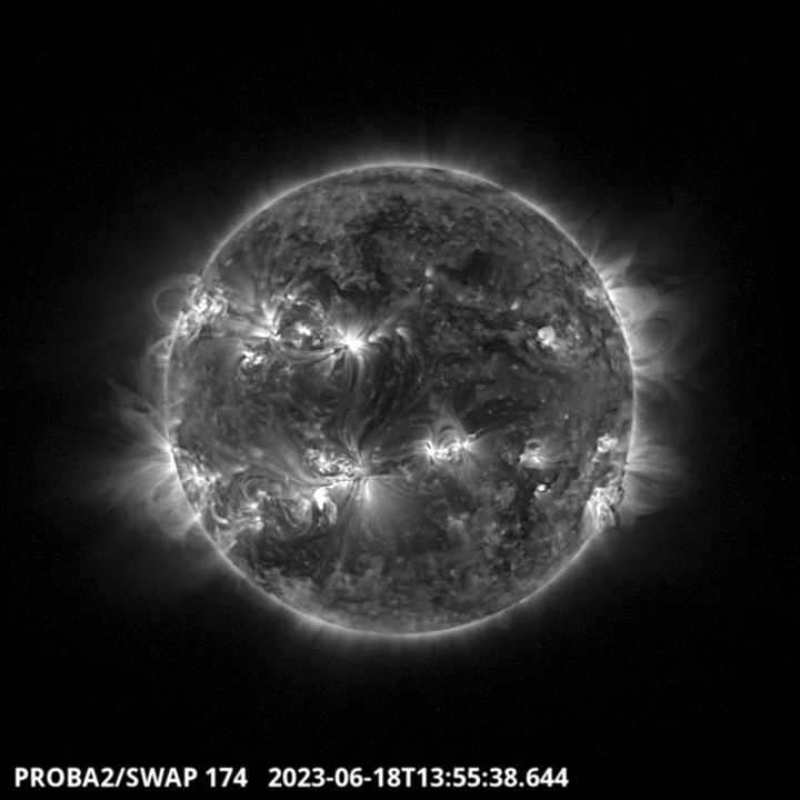
PROBA2 Observations (12 Jun 2023 - 18 Jun 2023)

Solar Activity

Solar flare activity fluctuated from low to moderate during the week.
In order to view the activity of this week in more detail, we suggest to go to the following website from which all the daily (normal and difference) movies can be accessed: https://proba2.oma.be/ssa
This page also lists the recorded flaring events.

A weekly overview movie (SWAP week 690) can be found here: https://proba2.sidc.be/swap/data/mpg/movies/weekly_movies/weekly_movie_2023_06_12.mp4.

Details about some of this week's events can be found further below.

If any of the linked movies are unavailable they can be found in the P2SC movie repository here: https://proba2.oma.be/swap/data/mpg/movies/.

Sunday June 18

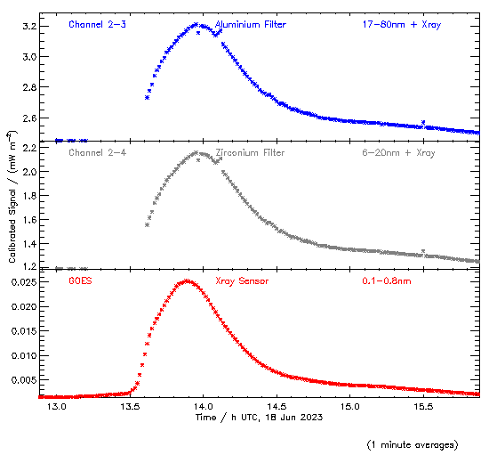
The largest flare of the week, an M2.5, was observed by LYRA (top panel) and SWAP (bottom panel). The flare occurred on 2023-Jun-18 (peak at 13:53 UT) in the south-western hemisphere, and it was associated with NOAA AR3336.
Find a SWAP movie of the event here: https://proba2.sidc.be/swap/movies/20230618_swap_movie.mp4.

International Sunspot Number by SILSO

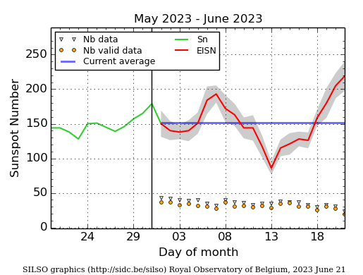
The daily Estimated International Sunspot Number (EISN, red curve with shaded error) derived by a simplified method from real-time data from the worldwide SILSO network. It extends the official Sunspot Number from the full processing of the preceding month (green line), a few days more than one solar rotation. The horizontal blue line shows the current monthly average. The yellow dots give the number of stations that provided valid data. Valid data are used to calculate the EISN. The triangle gives the number of stations providing data. When a triangle and a yellow dot coincide, it means that all the data is used to calculate the EISN of that day.

Noticeable Solar Events

DAY	BEGIN	MAX	END	LOC	XRAY	OP	10CM	TYPE	Cat	NOAA
16	0521	0530	0541		M1.0			VI/2		3337
16	1020	1038	1059		M1.0			III/1		3338
16	1952	1959	2007		M1.0				25	3331
18	0025	0031	0040		M1.3					3336
18	1325	1353	1414	S25E22	M2.5	2N		VI/2II/1		3336

LOC: approximate heliographic location	TYPE: radio burst type
XRAY: X-ray flare class	Cat: Catania sunspot group number
OP: optical flare class	NOAA: NOAA active region number
10CM: peak 10 cm radio flux

Geomagnetic Observations in Belgium

Local K-type magnetic activity index for Belgium based on data from Dourbes (DOU) and Manhay (MAB). Comparing the data from both measurement stations allows to reliably remove outliers from the magnetic data. At the same time the operational service availability is improved: whenever data from one observatory is not available, the single-station index obtained from the other can be used as a fallback system.
Both the two-station index and the single station indices are available here: http://ionosphere.meteo.be/geomagnetism/K_BEL/

The SIDC Space Weather Briefing

The Space Weather Briefing presented by the forecaster on duty from June 11 to 18. It reflects in images and graphs what is written in the Solar and Geomagnetic Activity report: https://www.stce.be/briefings/20230619_SWbriefing.pdf

If you need to access the movies, contact us: stce_coordination at stce.be

Review of Ionospheric Activity

The figure shows the time evolution of the Vertical Total Electron Content (VTEC) (in red) during the last week at three locations:
a) in the northern part of Europe(N 61deg E 5deg)
b) above Brussels(N 50.5deg, E 4.5 deg)
c) in the southern part of Europe(N 36 deg, E 5deg)
This figure also shows (in grey) the normal ionospheric behaviour expected based on the median VTEC from the 15 previous days.

The VTEC is expressed in TECu (with TECu=10^16 electrons per square meter) and is directly related to the signal propagation delay due to the ionosphere (in figure: delay on GPS L1 frequency).
The Sun's radiation ionizes the Earth's upper atmosphere, the ionosphere, located from about 60km to 1000km above the Earth's surface.The ionization process in the ionosphere produces ions and free electrons. These electrons perturb the propagation of the GNSS (Global Navigation Satellite System) signals by inducing a so-called ionospheric delay.

See http://stce.be/newsletter/GNSS_final.pdf for some more explanations ; for detailed information, see http://gnss.be/ionosphere_tutorial.php